April 27th, 2010 | 55 Comments
Gnuplot gives us the opportunity to produce great looking plots in a lot of different formats. Therefore it uses different output terminals that can produce output files or as in the last chapter display the output on your computer screen. In this tutorial we will cover the png, svg, postscript and epslatex terminals. Therefore we will use the same code as in the previous plot functions chapter. We already used the wxt terminal there which displays the result on the screen:
set terminal wxt size 350,262 enhanced font 'Verdana,10' persist
png, and svg terminal
The png and svg terminals produce more or less the same looking output as the wxt terminal, so you only have to replace the line for the wxt terminal with
set terminal pngcairo size 350,262 enhanced font 'Verdana,10'
set output 'introduction.png'
for png and with
set terminal svg size 350,262 fname 'Verdana' fsize 10
set output 'introduction.svg'
for svg to produce the same figures I have posted in the last chapter. You may have noticed that we use the pngcairo terminal. It exists also a png terminal, but it produces uglier output and doesn’t use the UTF-8 encoding the cairo library does. You may also have noticed that we set the size to a given x,y value. If we don’t do this, the default value of 640,480 is used. The enhanced option tells the terminals that they should interpret something like n_1 for us. But be aware that not all terminals handle the enhanced notation as mentioned in the gnuplot documentation.
Since we want to create an output file in both cases we have to specify one.
The png and svg terminals work very well to produce figures to use on the web as you can see on this page, but for scientific papers or other stuff written in LaTeX we would like to have figures in postscript or pdf format. I always create my pdf files of the plots from the postscript files, so I will cover only the postscript terminals in this introduction.
postscript terminal
gnuplot has a postscript terminal that can be used to produce figures in the eps format:
set terminal postscript eps enhanced color font 'Helvetica,10'
set output 'introduction.eps'
But this creates very tiny fonts, as stated in the documentation:
In eps mode the whole plot, including the fonts, is reduced to half of the default size.
So if we want to produce the same font and line width dimensions, we have to use this command:
set terminal postscript eps size 3.5,2.62 enhanced color \
    font 'Helvetica,20' linewidth 2
It tells the terminal the size in inches of the plot (note that this is the pixel dimension divided by 100) and uses a font size of 20 instead of 10. In addition to that it doubles the given line widths by a factor of 2.
Besides, the postscript terminal can’t handle all UTF-8 input characters and we have to use the enhanced mode to produce greek letter etc. But in opposite to the before mentioned terminals the enhanced mode will work fully for the postscript terminal.
set xlabel '{/Helvetica-Oblique x}'
set ylabel '{/Helvetica-Oblique y}'
set xtics ('-2{/Symbol p}' -2*pi,'-{/Symbol p}' -pi,0, \
    '{/Symbol p}' pi,'2{/Symbol p}' 2*pi)
plot f(x) title 'sin({/Helvetica-Oblique x})' with lines linestyle 1, \
Finally, we will get the following figure. Note, that I have converted the resulting eps file to png with Gimp using strong text and graphics antialiasing to show it here. But the overall looking should be the same as with the original eps file.
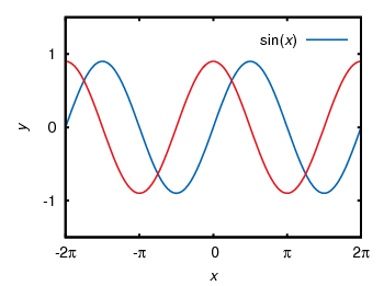
Fig. 1 Sinusoid plotted using the postscript terminal (code to produce this figure)
If we compare Fig. 1 to the original png file made with the pngcairo terminal (Fig. 2) we see that we still have some changes. We need to adjust the tic scales and line widths by hand to get exactly the same result. Note: the font is of course different, because we used another one.
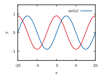
Fig. 2 Sinusoid plotted using the pngcairo terminal (code to produce this figure)
This means we should consider if want to create svg and png images or if we want to create eps and png images. In the first case we will use the wxt, svg and pngcairo terminals together.
In the second case we will use only the postscript terminal and create the png files using Gimp or some other image processor.
You may think the handling of symbols e.g. greek letters is very weird in the postscript terminal and you are probably right. But you can also write symbols in LaTeX notation, therefore you have to use the epslatex terminal.
epslatex terminal
If you have to write formulas or a scientific paper you are mostly interested in postscript/pdf or LaTeX output. The best way is to use both of them. That means to producing the lines etc. in the figure as a postscript image, but generate also a tex file that adds the text for us. The postscript image can be easily converted to a pdf using epstopdf if you needed a pdf version of the image. In order to create the tex file containing our figure labels we will use the epslatex terminal. Basically it has two working modes, a standalone mode that can produce a standalone postscript figure and the normal mode that produces a postscript figure and a tex file to include in your LaTeX document. I think the normal mode is the more common application so I will start with this.
For the normal mode we use the following terminal definition:
set terminal epslatex size 3.5,2.62 color colortext
set output 'introduction.tex'
color and colortext are needed if you have some colored labels, text etc. in your plot. size specifies the size of your plot in inches. You can specify the size alternatively in cm:
set terminal epslatex size 8.89cm,6.65cm color colortext
The easiest way is to specify the size to a value that corresponds with the needed one in your latex document. One way to get these values is to set your view to 100% in your pdf-viewer and measure the size of the area which should contain your figure. In Linux this is easily done using ScreenRuler.
Now we can write the labels etc. in LaTeX notation:
set xlabel '$x$'
set ylabel '$y$'
set format '$%g$'
set xtics ('$-2\pi$' -2*pi,'$-\pi$' -pi,0,'$\pi$' pi,'$2\pi$' 2*pi)
plot f(x) title '$\sin(x)$' with lines linestyle 1, \
Note that it is necessary to use the '' quotes and not "" in order to have interpreted your LaTeX code correctly.
If we run gnuplot on this file, it will generate a introduction.tex and a introduction-inc.eps file. In the LaTeX document we can then include the figure by:
\begin{figure}
    \input{introduction}
\end{figure}
Now our figure uses automatically the font and font size of our paper, but we still have to check that the line widths and tics have the size we want to. Also the size of the figure itself has to be correct in order to include it with the \input command without resizing it. Therefore we had to know the size of our figure before hand as mentioned above. Otherwise you should use the \resizebox command in LaTeX, but then it could be that your font size will be incorrect.
\begin{figure}
    \resizebox{\columnwidth}{!}{\input{introduction}}
\end{figure}
Note that you need the color package for colored labels. Therefore put \usepackage{color} in the preamble.
If you haven’t any LaTeX document, but want only to produce a figure with LaTeX labels, you can use the standalone mode.
Therefore exchange the above code with
set terminal epslatex size 3.5,2.62 standalone color colortext 10
set output 'introduction.tex'
The last value is the font size of the plot, which you don’t need if you want to include the figure in your LaTeX document.
To produce the standalone figure we have to run more than just the gnuplot command:
$ gnuplot introduction.gnu
$ latex introduction.tex
$ dvips -o introduction.ps introduction.dvi
The first command results in two files: introduction.tex with a LaTeX header and introduction-inc.eps which is the eps file of the figure without any text. The latex command combine the two to a single dvi file and dvips generates a postscript file. Finally I have converted the postscript file with Gimp and we will get this png file:
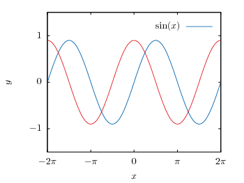
Fig. 3 Sinusoid plotted using the epslatex terminal (code to produce this figure)
If we compare this to Fig. 2 it is obvious that we have to fine tune the line widths and tics to get the same result as for the pngcairo terminal. In order to correct it we take the following values:
set border linewidth 2
set style line 1 linecolor rgb '#0060ad' linetype 1 linewidth 5
set style line 2 linecolor rgb '#dd181f' linetype 1 linewidth 5
set tics scale 1.25
Applying these settings will finally yield to a figure which looks like it should:
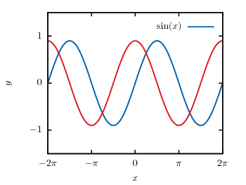
Fig. 4 Sinusoid plotted using the epslatex terminal with corrected line width and tics (code to produce this figure)
new as i am to computer i wish to request to a live tutorial in use of the terminal in downloading and plotting of light curves in astronomy. meanwhile these directions are very good and i appreciate them.
keep up.
thx.
Hi, I’m a huge fan of your page, after viewing how to use the esplatex terminal I’ve experienced some issues with setting the font size, apparently I need a ‘size*.clo’ file to modify the font size, I would really appreciate if you have a work around for this. Thanks!
[…] Gnuplotting: Output terminalshttp://www.gnuplotting.org/output-terminals/ […]
[…] output terminals […]
how to set terminals in a multi-plot?. I need eps image of multi-plot