Gnuplotting

Create scientific plots using gnuplot

June 24th, 2011 | No Comments

The filledcurves style is only available for 2d plots. But it can be used with some limitations with splot in 3d plots as well. In this entry we want to visualize an effect known from psychoacoustics, called comodulation masking release. The effect describes the possibility of our hearing system to perceive a masked tone (in this case at 700 Hz) easier in the presence of so called comodulated maskers present in other auditory filters. Comodulation describes the fact, that all maskers have the same envelope, as can be seen in Fig. 1.

CMR

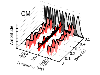
Fig. 1 Visualization of the comodulation masking release using splot and filledcurves (code to produce this figure, gfb_loop.gnu, gfb.dat, sig.dat, noise.dat)

First we start with the gammatone filters. The values for them are stored in the gfb.dat file as one column per filter. In order to apply different colors to different filters the style function sty(x) is defined. The data(x) function is defined to be able to plot the filters in a particular order. This will result in the nice effect of overlapping filters shown in Fig. 2.

sty(x) = x<7 ? 1 : x<10 ? 2 : x<12 ? 1 : x==12 ? 3 : x<15 ? 1 : \
    x==15 ? 2 : 1
data(x) = x<12 ? x : 29-x

The filter bank itself is plotted by the gfb_loop.gnu function. There the data are plotted first as filledcurves and then as a line. This two step mechanism has to be used, because the filledcurves style is not able to draw an extra line in 3d. Hence it has to be done in the extra gfb_loop.gnu function, because the simple for iteration only works for a single plot and is not able to plot the line around the filters.

# gfb_loop.gnu
splot 'gfb.dat' u 2:1:(column(data(i))) w filledcurves \
    ls sty(data(i)), \
      ''        u 2:1:(column(data(i))) ls 4
i = i+1
if (i<maxi) reread
CMR

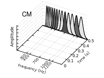
Fig. 2 Plotting gammatone filters with an extra loop file (code to produce this figure, gfb_loop.gnu, gfb.dat)

Thereafter the modulated noise and its envelope and the signal are plotted in different parts of the graph by explicitly giving the x position.
The result is shown in Fig. 1.

splot 'noise.dat' u  (300):1:2 ls 11, \
      ''          u  (300):1:3 ls 14, \
      ''          u  (400):1:2 ls 12, \
      ''          u  (400):1:3 ls 14, \
      ''          u  (700):1:2 ls 13, \
      ''          u  (700):1:3 ls 14, \
      ''          u (1000):1:2 ls 12, \
      ''          u (1000):1:3 ls 14, \
      ''          u (1100):1:2 ls 11, \
      ''          u (1100):1:3 ls 14
splot 'sig.dat'   u  (700):1:2 ls 14

May 6th, 2011 | 2 Comments

loudspeaker circle

Fig. 1 A circular loudspeaker array drawn with the object command (code to produce this figure, set_loudspeaker function)

In one of the last entries we have seen how to plot a loudspeaker with Gnuplot.
This time we will have a look at the case of setting more than one loudspeaker to your plot. Furthermore we allow the placement of the loudspeakers after entries in a data file.
Let us assume we have a data file containing the x position, y position and orientation phi of a single loudspeakers per line. Now we have to read the data with Gnuplot and set the objects according to the data. This can be done by a dummy plot, because by applying the plot command, variables can be stored. For the dummy plot we setting the output of the plot command to table and use /dev/null as the place to write the data.

# --- Read loudspeaker placement from data file
set table '/dev/null'
add_loudspeaker(x,y,phi) = sprintf(\
    'call "set_loudspeaker.gnu" "%f" "%f" "%f" "%f";',x,y,phi,0.2)
CMD = ''
plot 'loudspeaker_pos.dat' u 1:(CMD = CMD.add_loudspeaker($1,$2,$3))
eval(CMD)
unset table

The plot command now enables us to add the data from the file to the variable CMD, which is then executed by the eval command. To create the variable, the add_loudspeaker function creates a string with the data for every single line of the data file. The eval(CMD) calls the set_loudspeaker.gnu function once for every single data line, which corresponds to a single loudspeaker. The set_loudspeaker.gnu function itself does the same as we have done in the draw a single loudspeaker entry, but in addition it uses a rotation matrix to change the orientation of the single loudspeakers.

After having set the loudspeakers, we add some activity to three of the loudspeakers and finally get the result in Fig. 1.

# --- Plot loudspeaker activity
set parametric
fx(t,r,phi) = -1.5*cos(phi)+r*cos(t)
fy(t,r,phi) = -1.5*sin(phi)+r*sin(t)
set multiplot
set trange [-pi/6+pi/8:pi/6+pi/8]
plot for [n=1:3] fx(t,n*0.25,pi/8),fy(t,n*0.25,pi/8) w l ls 2
unset object
set trange [-pi/6-pi/8:pi/6-pi/8]
plot for [n=1:3] fx(t,n*0.25,-pi/8),fy(t,n*0.25,-pi/8) w l ls 2
set trange [-pi/6:pi/6]
plot for [n=1:3] fx(t,n*0.25,0),fy(t,n*0.25,0) w l ls 1
unset multiplot

The three waves before the desired loudspeakers are plotted within an iteration that effects the radius by using the for command. The unset object is executed after the first plot in the multiplot environment, because the loudspeakers should only be drawn once.