Gnuplotting

Create scientific plots using gnuplot

April 3rd, 2013 | 3 Comments

In one of the last posts, we came up with an updated data set representing the world. One way to plot this data set is with a 2D plot, as shown in Fig. 2. But if you compare the output with the one you see for example at Google Maps you will noticed a difference. That is due to the fact that Google uses the Mercator projection of the data. This projection preserves the angles around any point on the map, what is useful if you have a close look at some streets. The disadvantage of the Mercator projection is the inaccuracy of the sizes of the countries near to the poles. For example the size of Greenland is completely overemphasized as you can see in Fig. 1.

Mercator projection

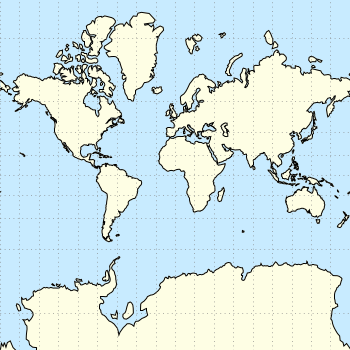
Fig. 1 Mercator projection of the world (code to produce this figure, data)

In order to achieve the Mercator projection, we apply the following function.

set angles degrees
mercator(latitude) = log( tan(180/4.0 + latitude/2.0) )
set yrange [-3.1:3.1]
plot 'world_110m.txt' u 1:(mercator($2)) w filledcu ls 2
Equirectangular projection

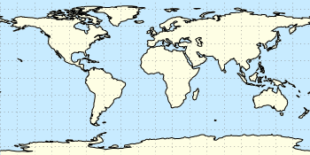
Fig. 2 Equirectangular projection of the world (code to produce this figure, data)

By just plotting the data as we have done for Fig. 2, we have the Equirectangular projection with constant spacing between the latitudes and meridians. The blue background color in the first two figures can be achieved directly with a terminal setting.

set terminal pngcairo size background '#c8ebff'
Heat map

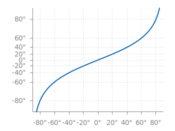
Fig. 3 Mapping of the Mercator projection (code to produce this figure)

In Fig. 3 the Mercator projection function is shown as an input-output-function of the latitude values. The placing of the latitude values on the y-axis can be easily done with a loop.

set ytics 0
do for [angle=-80:80:20] {
    set ytics add (sprintf('%.0f',angle) mercator(angle))
}

November 7th, 2012 | 6 Comments

Assume you have a data file describing a trajectory that you would like to animate like the spiral shown in Fig. 1.

moving spiral

Fig. 1 An animated spiral trajectory (code to produce this figure, data)

In order to create the animation we have to produce a set of png images and create the resulting gif animation with GIMP as shown in the Animation I – gif entry. Therefor, we have to tell gnuplot at which point of the data it has to stop for each image. This can be achieved by the every option. The point at the end of the line is just one data point. Here the start point and end point for every are just the same.

do for [ii=1:99] {
    splot 'spiral.txt' every ::1::ii w l ls 1, \
          'spiral.txt' every ::ii::ii w p ls 1
}

The downward spiral is created by running the loop in the other direction.

do for [ii=99:1:-1] {
    splot 'spiral.txt' every ::1::ii w l ls 1, \
          'spiral.txt' every ::ii::ii w p ls 1
}

By the way, I don’t know why the antialiasing of the output png images is not working in this example. If you have any idea, feel free to tell me.Assume you have a data file describing a trajectory that you would like to animate like the spiral shown in Fig. 1.

August 17th, 2012 | 7 Comments

As already mentioned gnuplot 4.6 overs an easier way to include loops in your code.
Here we are using it to create an animation of a set of head related impulse responses, which show differences in amplitude and arrival time at the left and right ear of a listener depending on the position of the source.

Fig. 1 Video animation of head related impulse responses (HRIRs) (code to produce this figure, data)

In comparison to the additional file for the loop in Animation I – gif, now all we need is this small code block.

do for [ii=1:181] {
    set output sprintf('hrir_frame%03.0f.png',ii)
    set multiplot layout 2,1
    [...]
    plot 'ir.txt' u ($1*1000):2*ii-1 w l ls 1
    [...]
    plot 'ir.txt' u ($1*1000):2*ii w l ls 1
    [...]
}

April 2nd, 2012 | 9 Comments

Since last month the new Gnuplot version 4.6 is officially available. There are a lot of interesting changes in this new version and we will cover the bigger ones within the next posts. Here we start with, in my opinion, the nicest new feature: block-structured conditions and loops.

Until 4.6 an iteration over different lines of code was only possible with the help of an extra file. This technique was used, for example, for the gif animation entry. There the loop was executed by

t = 0
end_time = 1
load 'bessel.plt'

with the file bessel.plt containing the code to execute within the loop

# bessel.plt
t = t + 0.02
outfile = sprintf('animation/bessel%03.0f.png',50*t)
set output outfile
splot u*sin(v),u*cos(v),bessel(u,t) w pm3d ls 1
if(t<end_time) reread;

This can now be reformulated in a much shorter way by applying the new do command and the block-structure given by the { }

do for [t=0:50] {
    outfile = sprintf('animation/bessel%03.0f.png',t)
    set output outfile
    splot u*sin(v),u*cos(v),bessel(u,t/50.0) w pm3d ls 1
}

Now there is no need for an additional file. The only thing to consider is the change of the index t, because for the for-loop t has to be an integer.

The block-structure can in the same way be applied to the if-statement.