Gnuplotting

Create scientific plots using gnuplot

June 23rd, 2014 | 8 Comments

Occasionally it is a good idea to create a zoom of some part of your main plot, especially if you have a small part of your plot where the data is hiding each other.

Including a zoom with multiplot

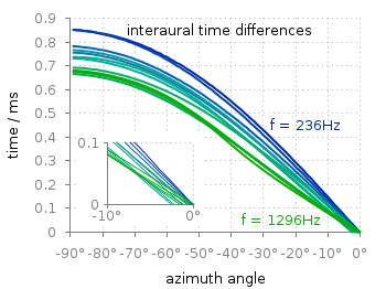
Fig. 1 Including a zoom into your figure to emphasize some data. (code to produce this figure, data)

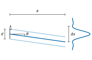
In Fig. 1 the interaural time difference between a sound signal reaching the two ears of a listener is plotted with different colors for different frequencies. The data is very dense around 0°, so we include a zoom into this region in the same figure at a free place.

This can be done via multiplot and the plotting of the same data in a smaller figure.

set origin 0.12,0.17
set size 0.45,0.4
set xrange [-10:0]
set yrange [0:0.1]
plot for [n=2:13] 'itd.txt' u 1:(column(n)*1000) w lines ls n

The tricky part is that we have a grid in our main figure and if we do nothing the grid will also be visible in the zoomed in version as shown in Fig. 2.

Including a zoom with multiplot without grid correction

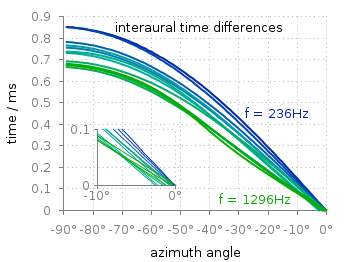
Fig. 2 Including a zoom into your figure, without correcting the grid. (code to produce this figure, data)

To avoid this we have to hide the grid in the background of the zoomed graph. This is done with the trick of placing an empty white rectangle at the place the zoom plot should appear in the figure.

set object 1 rect from -88,0.03 to -49,0.41
set object 1 rect fc rgb 'white' fillstyle solid 0.0 noborder

This will then finally lead to the desired result presented in Fig. 1.

February 21st, 2014 | 5 Comments

For the measurement of distances T-shaped arrows are often used to highlight the length. In gnuplot there is an easy way to achieve this.

Diffraction on a slit

Fig. 1 Diffraction of light for a slit with the length d. (code to produce this figure)

Have a look at Fig. 1 which tries to explain the diffraction phenomenon of a slit with the length d. At a distance a the diffraction pattern is drawn. The different distances, the distance between the first minima of the diffraction pattern, and the wave length are indicated by T-shaped arrows. This kind of arrays can be achieved in gnuplot with the following code.

Theads = 'heads size 0.5,90 front ls 201'
set arrow from -24,-2 to -24, 2       @Theads
set arrow from -22, 2 to -21.44,1.92  @Theads
set arrow from 1.5,-pi to 1.5,pi      @Theads
set arrow from -22,2.5*pi to 0,2.5*pi @Theads

Here, 90 is the relevant entry after size as it describes the opening angle of the arrow head.
In addition, an open circle is drawn to indicate the angle θ. This is achieved by specifying the opening angle for the circle object.

set object circle at -22,0 size 6 arc [-8:0]

May 6th, 2011 | 2 Comments

loudspeaker circle

Fig. 1 A circular loudspeaker array drawn with the object command (code to produce this figure, set_loudspeaker function)

In one of the last entries we have seen how to plot a loudspeaker with Gnuplot.
This time we will have a look at the case of setting more than one loudspeaker to your plot. Furthermore we allow the placement of the loudspeakers after entries in a data file.
Let us assume we have a data file containing the x position, y position and orientation phi of a single loudspeakers per line. Now we have to read the data with Gnuplot and set the objects according to the data. This can be done by a dummy plot, because by applying the plot command, variables can be stored. For the dummy plot we setting the output of the plot command to table and use /dev/null as the place to write the data.

# --- Read loudspeaker placement from data file
set table '/dev/null'
add_loudspeaker(x,y,phi) = sprintf(\
    'call "set_loudspeaker.gnu" "%f" "%f" "%f" "%f";',x,y,phi,0.2)
CMD = ''
plot 'loudspeaker_pos.dat' u 1:(CMD = CMD.add_loudspeaker($1,$2,$3))
eval(CMD)
unset table

The plot command now enables us to add the data from the file to the variable CMD, which is then executed by the eval command. To create the variable, the add_loudspeaker function creates a string with the data for every single line of the data file. The eval(CMD) calls the set_loudspeaker.gnu function once for every single data line, which corresponds to a single loudspeaker. The set_loudspeaker.gnu function itself does the same as we have done in the draw a single loudspeaker entry, but in addition it uses a rotation matrix to change the orientation of the single loudspeakers.

After having set the loudspeakers, we add some activity to three of the loudspeakers and finally get the result in Fig. 1.

# --- Plot loudspeaker activity
set parametric
fx(t,r,phi) = -1.5*cos(phi)+r*cos(t)
fy(t,r,phi) = -1.5*sin(phi)+r*sin(t)
set multiplot
set trange [-pi/6+pi/8:pi/6+pi/8]
plot for [n=1:3] fx(t,n*0.25,pi/8),fy(t,n*0.25,pi/8) w l ls 2
unset object
set trange [-pi/6-pi/8:pi/6-pi/8]
plot for [n=1:3] fx(t,n*0.25,-pi/8),fy(t,n*0.25,-pi/8) w l ls 2
set trange [-pi/6:pi/6]
plot for [n=1:3] fx(t,n*0.25,0),fy(t,n*0.25,0) w l ls 1
unset multiplot

The three waves before the desired loudspeakers are plotted within an iteration that effects the radius by using the for command. The unset object is executed after the first plot in the multiplot environment, because the loudspeakers should only be drawn once.

March 15th, 2011 | No Comments

As you all know Gnuplot is able to add arrows or labels to your plot. But it can even add more complicated objects, by using the object command. You can choose if you want to add a rectangle, ellipse, circle, or polygon. Here we want to add a loudspeaker to our plot, hence we choose the polygon.

loudspeaker

Fig. 1 A loudspeaker drawn with the object command (code to produce this figure)

For a polygon you have to specify the points the polygon should combine. The following points will result in a shape of the desired loudspeaker.

a = 1.0/3
set object 1 polygon from \
    -1, 1 to \
     0, 1 to \
     0, a to \
     1, 1 to \
     1,-1 to \
     0,-a to \
     0,-1 to \
    -1,-1 to \
    -1, 1

After this we do some fine tuning on the appearance of the object and remove all borders and tics from the plot.

unset border
unset tics
set object 1 fc rgb '#000000' fillstyle solid lw 0

In order to draw the loudspeaker we need a plot command. For this we use the parametric mode to draw parts of circles with different radii. Here I will only present the used functions, for an explanation of the parametric mode have a look at the Understand parametric mode entry.

set trange [-pi/6:pi/6]
fx(t,r) = r*cos(t)
fy(t,r) = r*sin(t)