parametric « Gnuplotting

December 18th, 2012 | 48 Comments

More than a year ago, we draw a map of the world with gnuplot. But it has been pointed out the low resolution of the map data. For example, Denmark is totally missing in the original data file. The good thing is, there is other data available in the web. In this entry we will consider how to use the physical coastline data from http://www.naturalearthdata.com/downloads/ together with gnuplot.

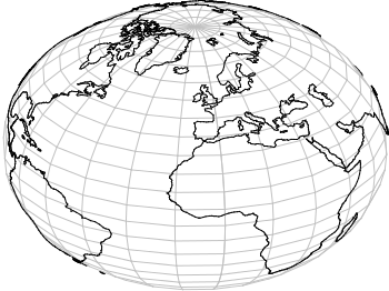
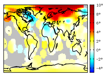
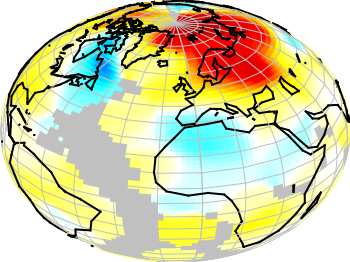
Fig. 1 Plot of the world with the new data file and a resolution of 1:110m (code to produce this figure, data)

At the download page, three different resolutions of the data are available with a scale of 1:10m, 1:50m, or 1:110m. The data itself is stored as shape files on naturalearthdata.com. Hence I wrote a script that converts the data first to a csv file using the ogr2ogr program. Afterwards the data is shaped with sed into the form of the original world.dat file.
Here are the resulting files:

Fig.1 shows the result for a resolution of 1:110m. Note that we have to use linetype instead of linestyle in gnuplot 4.6 in order to set the colors of the grid and coast line.

In order to compare the different resolutions of the coast line files, we plot only the part of the map where Denmark is located (which is completely missing in the original data).
Here is the example code for a scale of 1:110m.

set xrange [7.5:13]
set yrange [54.5:58]
plot 'world_110m.txt' with filledcurves ls 1, \
    '' with l ls 2

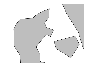
Fig. 2 A plot of Denmark at a resolution of 1:110m. (code to produce this figure, data)

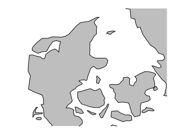
Fig. 3 A plot of Denmark at a resolution of 1:50m. (code to produce this figure, data)

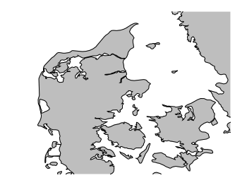
Fig. 4 A plot of Denmark at a resolution of 1:10m. (code to produce this figure, data)

Tags: 4.6, data, hidden3d, linestyle, linetype, parametric

July 29th, 2011 | 5 Comments

In one post we have used the parametric plot option to plot the world. Here we want to add some temperature data as a heat map to the world plots. The data show the temperature anomalies of the year 2005 in comparison to the baseline 1951-1980 and is part of the GISTEMP data set.

Fig. 1 A 2D heat map of the temperature anomalies in 2005 to the baseline 1951-1980 (code to produce this figure, temperature data, world data)

The first problem you face, if you want to create a heat map, is that the data has to be in a specific format shown in the Gnuplot example page for heat maps. Therefore we first arrange the data and end up with this temperature anomalies file. Unknown data points are given by 9999.0.

In order to plot this data to the 2D world map we have to add a reasonable cbrange and a color palette and the plot command for the map:

set cbrange [-5:10]
set palette defined (0 "blue",17 "#00ffff",33 "white",50 "yellow",\
    66 "red",100 "#990000",101 "grey")
plot 'temperature.dat' u 2:1:3 w image, \
     'world.dat' with lines linestyle 1

The trick with the wide range from 0 to 101 for the color bar is chosen in order to use grey for the undefined values (9999.0) without seeing the grey color in the color bar. The result is shown in Fig. 1.

Fig. 2 A 3D heat map of the temperature anomalies in 2005 to the baseline 1951-1980 (code to produce this figure, temperature data, world data)

The same data can easily be applied to the 3D plot of the world. We have to add front to the hidden3d command in order to make the black world lines visible. In addition the radius must be given explicitly as third column to the plot command for the temperature data.

set hidden3d front
splot 'temperature.dat' u 2:1:(1):3 w pm3d, \
      r*cos(v)*cos(u),r*cos(v)*sin(u),r*sin(v) w l ls 2, \
      'world.dat' u 1:2:(1) w l ls 1

The result is shown in Fig. 2.

Tags: data, hidden3d, parametric, pm3d, sphere

June 7th, 2011 | 6 Comments

A Klein bottle is a non-orientable surface, which has no defined left and right, as stated on Wikipedia. There we can also find a Gnuplot plot of the bottle, which we want to fine-tune a little bit in order to reach the result in Fig. 1.

Fig. 1 Klein bottle (code to produce this figure)

In order to reach Fig. 1 we start with the definition of the parametric functions given in Wikipedia and do a simple pm3d plot with them.

set parametric
x(u,v)= v<2*pi ? (2.5-1.5*cos(v))*cos(u) : \
        v<3*pi ? -2+(2+cos(u))*cos(v)    : \
                 -2+2*cos(v)-cos(u)
y(u,v)= v<2*pi ? (2.5-1.5*cos(v))*sin(u) : \
                sin(u)
z(u,v)= v<pi   ? -2.5*sin(v)             : \
        v<2*pi ? 3*v-3*pi                : \
        v<3*pi ? (2+cos(u))*sin(v)+3*pi  : \
                 -3*v+12*pi
splot x(u,v),y(u,v),-z(u,v) w pm3d

The result is shown in Fig. 2.

Fig. 2 Klein bottle plotted only with pm3d (code to produce this figure)

Now we add some lines to the surface and hide parts, which are not visible in 3d.

set pm3d depthorder hidden3d 1
set hidden3d

Here the depthorder option takes care of the right positioning of the bottleneck going back into the bottle, which is not correct in Fig. 2. The hidden3d 1 option draws lines in the right order for a correctly looking 3d plot using line style 1. The additional set hidden3d command takes care of showing only those lines that are visible in 3d. These options will result in Fig. 3.

Fig. 3 Klein bottle plotted only with pm3d and hidden3d (code to produce this figure)

In order to reach at Fig. 1 we just have to set the surface to be transparent, which can be done by the set style fill command.

set style fill transparent solid 0.65

Tags: depthorder, hidden3d, parametric, pm3d, splot, transparent

May 6th, 2011 | 2 Comments

Fig. 1 A circular loudspeaker array drawn with the object command (code to produce this figure, set_loudspeaker function)

In one of the last entries we have seen how to plot a loudspeaker with Gnuplot.
This time we will have a look at the case of setting more than one loudspeaker to your plot. Furthermore we allow the placement of the loudspeakers after entries in a data file.
Let us assume we have a data file containing the x position, y position and orientation phi of a single loudspeakers per line. Now we have to read the data with Gnuplot and set the objects according to the data. This can be done by a dummy plot, because by applying the plot command, variables can be stored. For the dummy plot we setting the output of the plot command to table and use /dev/null as the place to write the data.

# --- Read loudspeaker placement from data file
set table '/dev/null'
add_loudspeaker(x,y,phi) = sprintf(\
    'call "set_loudspeaker.gnu" "%f" "%f" "%f" "%f";',x,y,phi,0.2)
CMD = ''
plot 'loudspeaker_pos.dat' u 1:(CMD = CMD.add_loudspeaker($1,$2,$3))
eval(CMD)
unset table

The plot command now enables us to add the data from the file to the variable CMD, which is then executed by the eval command. To create the variable, the add_loudspeaker function creates a string with the data for every single line of the data file. The eval(CMD) calls the set_loudspeaker.gnu function once for every single data line, which corresponds to a single loudspeaker. The set_loudspeaker.gnu function itself does the same as we have done in the draw a single loudspeaker entry, but in addition it uses a rotation matrix to change the orientation of the single loudspeakers.

After having set the loudspeakers, we add some activity to three of the loudspeakers and finally get the result in Fig. 1.

# --- Plot loudspeaker activity
set parametric
fx(t,r,phi) = -1.5*cos(phi)+r*cos(t)
fy(t,r,phi) = -1.5*sin(phi)+r*sin(t)
set multiplot
set trange [-pi/6+pi/8:pi/6+pi/8]
plot for [n=1:3] fx(t,n*0.25,pi/8),fy(t,n*0.25,pi/8) w l ls 2
unset object
set trange [-pi/6-pi/8:pi/6-pi/8]
plot for [n=1:3] fx(t,n*0.25,-pi/8),fy(t,n*0.25,-pi/8) w l ls 2
set trange [-pi/6:pi/6]
plot for [n=1:3] fx(t,n*0.25,0),fy(t,n*0.25,0) w l ls 1
unset multiplot

The three waves before the desired loudspeakers are plotted within an iteration that effects the radius by using the for command. The unset object is executed after the first plot in the multiplot environment, because the loudspeakers should only be drawn once.

Tags: call, circle, data, for, iteration, object, parametric, polygon, table

March 15th, 2011 | No Comments

As you all know Gnuplot is able to add arrows or labels to your plot. But it can even add more complicated objects, by using the object command. You can choose if you want to add a rectangle, ellipse, circle, or polygon. Here we want to add a loudspeaker to our plot, hence we choose the polygon.

Fig. 1 A loudspeaker drawn with the object command (code to produce this figure)

For a polygon you have to specify the points the polygon should combine. The following points will result in a shape of the desired loudspeaker.

a = 1.0/3
set object 1 polygon from \
    -1, 1 to \
     0, 1 to \
     0, a to \
     1, 1 to \
     1,-1 to \
     0,-a to \
     0,-1 to \
    -1,-1 to \
    -1, 1

After this we do some fine tuning on the appearance of the object and remove all borders and tics from the plot.

unset border
unset tics
set object 1 fc rgb '#000000' fillstyle solid lw 0

In order to draw the loudspeaker we need a plot command. For this we use the parametric mode to draw parts of circles with different radii. Here I will only present the used functions, for an explanation of the parametric mode have a look at the Understand parametric mode entry.

set trange [-pi/6:pi/6]
fx(t,r) = r*cos(t)
fy(t,r) = r*sin(t)

Tags: border, object, parametric, polygon, tics

July 11th, 2010 | 5 Comments

In the Gnuplot demo files folder that comes with your Gnuplot installation exists the file world.dat which contains data in order to plot a map of the world. Therefore we remove the key from the figure and set a grid (the dashed line in Fig. 1). Also we remove the tics by setting the format to nothing and the scale to zero. We could also remove the tics with unset tics, but the grid depends on the tics positions. After that we just plot the data:

unset key
set grid
set format ''
set tics scale 0
plot 'world.dat' with lines linestyle 1

Fig. 1 A 2D plot of the world (code to produce this figure)

Here you can see a problem of the svg terminal of Gnuplot: it can’t produce dashed lines. In order to fix this, we can use Inkscape and open the svg file. Then pressing CRTL+F and type gray into the Style field and hit Enter. Now all the grid lines should be selected and you can set their stroke style to dashed by typing CRTL+Shift+F and choose one under Dashes. Doing so will lead to a figure shown in Fig. 2.

Fig. 2 The 2D plot of the world edited with Inkscape

We can also easily draw a whole globe in 3D from the given data. Therefore we first add a gray line style, unset the border and arrange the figure margins.

set style line 2 lc rgb '#c0c0c0' lt 1 lw 2
unset border
set lmargin screen 0
set bmargin screen 0
set rmargin screen 1
set tmargin screen 1

The 3D plot needs a little more settings. We have to tell Gnuplot to map the data on a sphere and using angle values in degree. Also we want to have a non transparent world, therefore we need hidden3d. We arrange the appeareance of the plot by setting the xy-plane to the lowest z value in order to avoid an
offset between the lowest z vlaue an the xy-plane. To have Europe in the center we set also the viewport.

set mapping spherical
set angles degrees
set hidden3d
set xyplane at -1
set view 56,81

For the grid we have to remove the set grid command, because it doesn’t work with splot. So we draw the grid by our own using the parametric mode and finally plot the whole globe:

set parametric
set isosamples 25
set urange[0:360]
set vrange[-90:90]
splot cos(v)*cos(u),cos(v)*sin(u),sin(v) with lines linestyle 2, \
      'world.dat' with lines linestyle 1

Fig. 3 A 3D plot of the world (code to produce this figure)

As you can see we have some problems with the data for Africa which lies behind the grid at some points. To avoid this and to make the grid dashed again we draw a grid with tinier radius and use Inkscape.

r = 0.99
splot r*cos(v)*cos(u),r*cos(v)*sin(u),r*sin(v) with lines \
      linestyle 2, \

In order to select the grid in Inkscape we have to search after the Style blue for some strange reason (on another PC green was the right color to search). You may have a look at the xml data to figure this out. Therefore under Edit you will find XML Editor. We not only set the stroke style to dashed we also lowered the selected objects
to avoid that any line of the grid covered a black world line. Having done all that we will finally get the nice globe in Fig. 4.

Fig. 4 The 3D plot of the world edited with Inkscape

Tags: dashed, data, grid, parametric, svg

June 4th, 2010 | 6 Comments

If one have a coordinate system with n-dimension, then one of the dimensions can be expressed by the n-1 other dimensions, e.g. z = f(x,y).
But if you want to plot functions that are defined in polar coordinates, e.g. a sphere, they are complicated to define with z = f(x,y). But Gnuplot offers you a way to handle this type of functions by using its parametric mode. In parametric mode the functions are expressed in angular coordinates t or u,v dependend on the dimensions of your plot.

2D case

In the 2D case we have only one free dimension:

y = f(x)   =>   x = fx(t), y = fy(t)

In Fig. 1 we see the connections between the angular coordinate t and radius r and x,y that is given by

x = r cos(t)
y = r cos(π/2-t) = r sin(t)

Fig. 1 Connection between Gnuplots parametric variable t and x,y (code to produce this figure)

Using the result from above it is very easy to plot a circle:

set parametric
set trange [0:2*pi]
# Parametric functions for a circle
fx(t) = r*cos(t)
fy(t) = r*sin(t)
plot fx(t),fy(t)

Fig. 2 Plot of a circle using Gnuplots parametric mode (code to produce this figure)

3D case

In three dimensions we have the case:

z = f(x,y)   =>   x = fx(u,v), y = fy(u,v), z = fz(u,v)

In Fig. 3 we see the connection between the two angular variables u (that is t in the 2D case), v and the radius r:

x = r cos(v) cos(u)
y = r cos(v) sin(u)
z = r sin(u)

Fig. 3 Connection between Gnuplots parametric variables u,v and x,y,z (code to produce this figure)

Using the parametric variables u,v it is very easy to draw a sphere or a piece of a sphere:

set parametric
set urange [0:3.0/2*pi]
set vrange [-pi/2:pi/2]
# Parametric functions for the sphere
fx(v,u) = r*cos(v)*cos(u)
fy(v,u) = r*cos(v)*sin(u)
fz(v)   = r*sin(v)
splot fx(v,u),fy(v,u),fz(v)

The result is shown in Fig. 4. Note that we have to use 3.0/2, because 3/2 is 1 for Gnuplot!

Fig. 4 Plot of a sphere using Gnuplots parametric mode (code to produce this figure)

Tags: circle, parametric, sphere

Gnuplotting

Plotting the world revisited

Heat maps

Klein bottle

Object placement using a data file

Drawing a loudspeaker

Plotting the world

Understand parametric plotting

2D case

3D case

Gnuplot Links