September 3rd, 2016 | 2 Comments
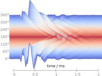
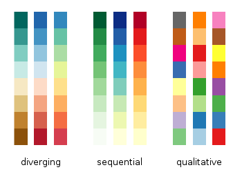
Matplotlib has four new colormaps called viridis, plasma, magma, and inferno. Especially viridis you might have seen already as this will be the new default in Matplotlib 2.0. They are freely available and now also included in the gnuplot-palettes repository on github. They are well designed to be perceptually uniform and friendly for common forms of colorblindness, so they should be save to use as your default colormap. Personally I would not recommend them for every kind of plot as they are a little dark if you have large areas with low values in your plot.
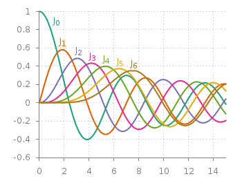
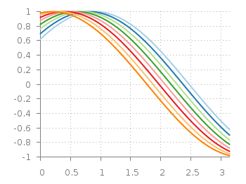
As usual in the gnuplot-palettes repository they are accompanied by line style definitions using the palette colors.
# viridis
set style line  1 lt 1 lc rgb '#440154' # dark purple
set style line  2 lt 1 lc rgb '#472c7a' # purple
set style line  3 lt 1 lc rgb '#3b518b' # blue
set style line  4 lt 1 lc rgb '#2c718e' # blue
set style line  5 lt 1 lc rgb '#21908d' # blue-green
set style line  6 lt 1 lc rgb '#27ad81' # green
set style line  7 lt 1 lc rgb '#5cc863' # green
set style line  8 lt 1 lc rgb '#aadc32' # lime green
set style line  9 lt 1 lc rgb '#fde725' # yellow
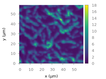
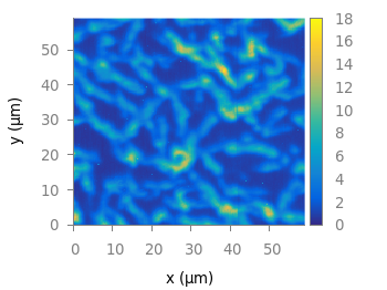
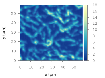
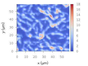
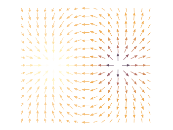
Fig. 1 Photoluminescence yield plotted with the viridis colormap from Matplotlib (code to produce this figure, viridis.pal, data)
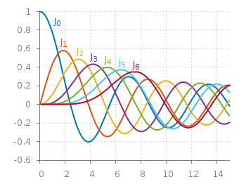
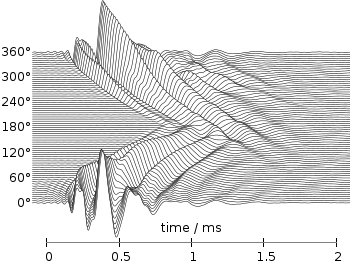
# plasma
set style line  1 lt 1 lc rgb '#0c0887' # blue
set style line  2 lt 1 lc rgb '#4b03a1' # purple-blue
set style line  3 lt 1 lc rgb '#7d03a8' # purple
set style line  4 lt 1 lc rgb '#a82296' # purple
set style line  5 lt 1 lc rgb '#cb4679' # magenta
set style line  6 lt 1 lc rgb '#e56b5d' # red
set style line  7 lt 1 lc rgb '#f89441' # orange
set style line  8 lt 1 lc rgb '#fdc328' # orange
set style line  9 lt 1 lc rgb '#f0f921' # yellow
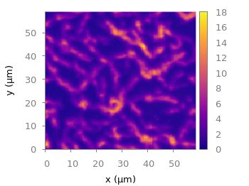
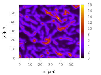
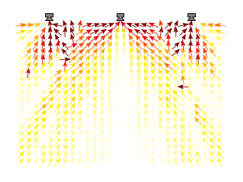
Fig. 2 Photoluminescence yield plotted with the plasma colormap from Matplotlib (code to produce this figure, plasma.pal, data)
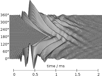
# magma
set style line  1 lt 1 lc rgb '#000004' # black
set style line  2 lt 1 lc rgb '#1c1044' # dark blue
set style line  3 lt 1 lc rgb '#4f127b' # dark purple
set style line  4 lt 1 lc rgb '#812581' # purple
set style line  5 lt 1 lc rgb '#b5367a' # magenta
set style line  6 lt 1 lc rgb '#e55964' # light red
set style line  7 lt 1 lc rgb '#fb8761' # orange
set style line  8 lt 1 lc rgb '#fec287' # light orange
set style line  9 lt 1 lc rgb '#fbfdbf' # light yellow
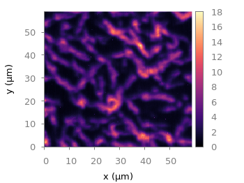
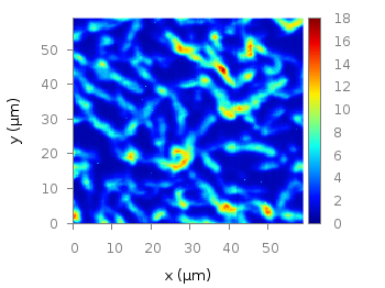
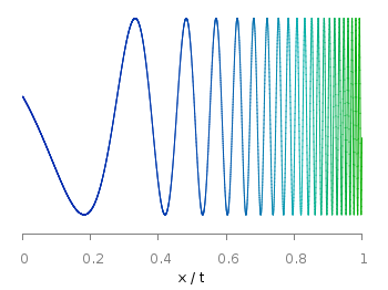
Fig. 3 Photoluminescence yield plotted with the magma colormap from Matplotlib (code to produce this figure, magma.pal, data)
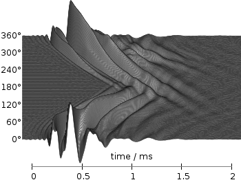
# inferno
set style line  1 lt 1 lc rgb '#000004' # black
set style line  2 lt 1 lc rgb '#1f0c48' # dark purple
set style line  3 lt 1 lc rgb '#550f6d' # dark purple
set style line  4 lt 1 lc rgb '#88226a' # purple
set style line  5 lt 1 lc rgb '#a83655' # red-magenta
set style line  6 lt 1 lc rgb '#e35933' # red
set style line  7 lt 1 lc rgb '#f9950a' # orange
set style line  8 lt 1 lc rgb '#f8c932' # yellow-orange
set style line  9 lt 1 lc rgb '#fcffa4' # light yellow
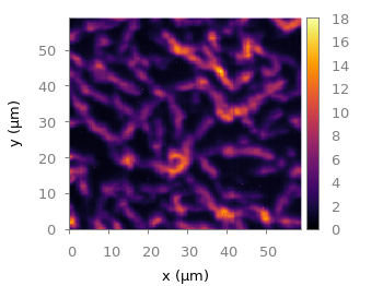
Fig. 4 Photoluminescence yield plotted with the inferno colormap from Matplotlib (code to produce this figure, inferno.pal, data)