colormap « Gnuplotting

September 23rd, 2016 | 4 Comments

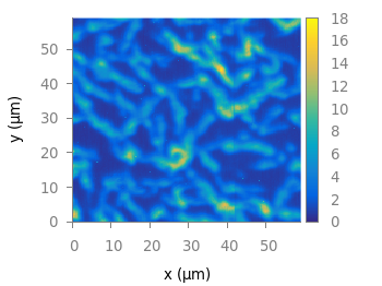
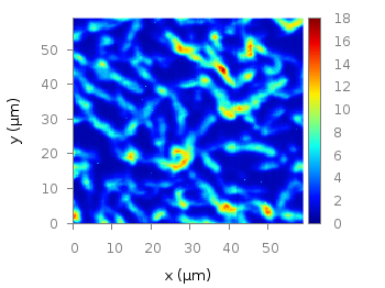
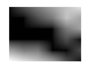
Suppose you have a large circular container filled with sand and measure its density at different positions. Now the goal is to display your measurements as a heat map extrapolated from your measurements, but limiting that heat map to the inner part of the container as shown in Fig. 1.

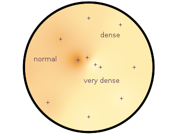
Fig. 1 Sand density measured at different positions in a circular container (code to produce this figure, sand.pal, data)

The underlying measurements are provided in the following format:

# sand_density_orig.txt
#1      2        3        4      5       6
#prob   x        y        z      density description
"E01"   0.00000 -1.14161 -0.020  0.7500  "dense"
"E02"  -0.94493 -0.81804 -0.020  0.5753  "normal"
"E03"   0.75306 -0.72000 -0.020  0.7792  "dense"
...

Those data points have to be extrapolated onto a grid for the heat map, which can be achieved by the following commands.

set view map
set pm3d at b map
set dgrid3d 200,200,2
splot "sand_density1.txt" u 2:3:5

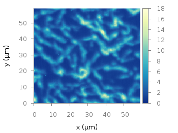
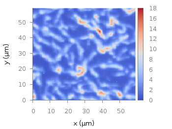
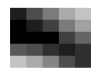
Fig. 2 shows the result which has two problems. The grid data is limited to the boundary given by the measurement points. In addition, the grid is always rectangular in size and not circular.

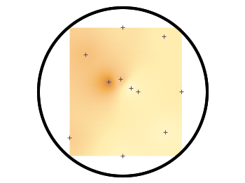
Fig. 2 Sand density measured at different positions in a circular container (code to produce this figure, sand.pal, data)

To overcome the first problem you have to add four additional points to the original data in order to stretch the grid boundary to the radius of the container. For that you have to come up with some reasonable extrapolation from the existing points. I did this in a very simple way by a mixture of linear interpolation or using the value of the nearest point. If you want to do the same with your data set you should maybe spent a little bit more effort on this.

# sand_density.txt
#1      2        3        4      5       6
#prob   x        y        z      density description
"E01"   0.00000 -1.14161 -0.020  0.7500  "dense"
...
"xmin" -1.50000  0.00000 -0.050  0.5508  "dummy"
"xmax"  1.50000  0.00000 -0.050  0.6634  "dummy"
"ymin"  0.00000 -1.50000 -0.050  0.7500  "dummy"
"ymax"  0.00000  1.50000 -0.050  0.6315  "dummy"

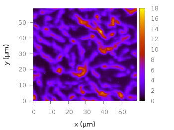
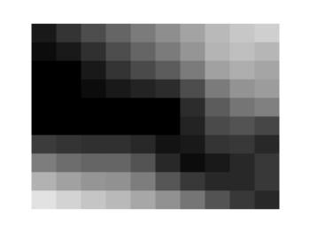
If you plot those modified data set you will get Fig. 3.

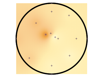
Fig. 3 Sand density measured at different positions in a circular container (code to produce this figure, sand.pal, data)

In order to limit the heat map to a circle you first extrapolate the grid using dgrid3d and store the data in a new file.

set table "tmp.txt"
set dgrid3d 200,200,2
splot "sand_density2.txt" u 2:3:5
unset table

Afterwards a function is defined in order to limit the points to the inner of the circle and plot the data from the temporary file.

circle(x,y,z) = sqrt(x**2+y**2)>r ? NaN : z
plot "tmp.txt" u 1:2:(circle($1,$2,$3)) w image

Finally a few labels and the original measurement points are added. The manually added points like xmin are removed by a smaller radius value. The result is then the nice circular heat map in Fig. 1.

r = 1.49 # make radius smaller to exclude interpolated edge points
set label 'normal' at -1,0.2 center front tc ls 1
set label 'dense' at 0.5,0.75 center front tc ls 1
set label 'very dense' at 0.3,-0.3 center front tc ls 1
plot "sand_density.txt" \
         u (circle($2,$3,$2)):(circle($2,$3,$3)) w p ls 1

Tags: circle, colormap, dgrid3d, grid, image

September 3rd, 2016 | 2 Comments

Matplotlib has four new colormaps called viridis, plasma, magma, and inferno. Especially viridis you might have seen already as this will be the new default in Matplotlib 2.0. They are freely available and now also included in the gnuplot-palettes repository on github. They are well designed to be perceptually uniform and friendly for common forms of colorblindness, so they should be save to use as your default colormap. Personally I would not recommend them for every kind of plot as they are a little dark if you have large areas with low values in your plot.

As usual in the gnuplot-palettes repository they are accompanied by line style definitions using the palette colors.

# viridis
set style line  1 lt 1 lc rgb '#440154' # dark purple
set style line  2 lt 1 lc rgb '#472c7a' # purple
set style line  3 lt 1 lc rgb '#3b518b' # blue
set style line  4 lt 1 lc rgb '#2c718e' # blue
set style line  5 lt 1 lc rgb '#21908d' # blue-green
set style line  6 lt 1 lc rgb '#27ad81' # green
set style line  7 lt 1 lc rgb '#5cc863' # green
set style line  8 lt 1 lc rgb '#aadc32' # lime green
set style line  9 lt 1 lc rgb '#fde725' # yellow

Fig. 1 Photoluminescence yield plotted with the viridis colormap from Matplotlib (code to produce this figure, viridis.pal, data)

# plasma
set style line  1 lt 1 lc rgb '#0c0887' # blue
set style line  2 lt 1 lc rgb '#4b03a1' # purple-blue
set style line  3 lt 1 lc rgb '#7d03a8' # purple
set style line  4 lt 1 lc rgb '#a82296' # purple
set style line  5 lt 1 lc rgb '#cb4679' # magenta
set style line  6 lt 1 lc rgb '#e56b5d' # red
set style line  7 lt 1 lc rgb '#f89441' # orange
set style line  8 lt 1 lc rgb '#fdc328' # orange
set style line  9 lt 1 lc rgb '#f0f921' # yellow

Fig. 2 Photoluminescence yield plotted with the plasma colormap from Matplotlib (code to produce this figure, plasma.pal, data)

# magma
set style line  1 lt 1 lc rgb '#000004' # black
set style line  2 lt 1 lc rgb '#1c1044' # dark blue
set style line  3 lt 1 lc rgb '#4f127b' # dark purple
set style line  4 lt 1 lc rgb '#812581' # purple
set style line  5 lt 1 lc rgb '#b5367a' # magenta
set style line  6 lt 1 lc rgb '#e55964' # light red
set style line  7 lt 1 lc rgb '#fb8761' # orange
set style line  8 lt 1 lc rgb '#fec287' # light orange
set style line  9 lt 1 lc rgb '#fbfdbf' # light yellow

Fig. 3 Photoluminescence yield plotted with the magma colormap from Matplotlib (code to produce this figure, magma.pal, data)

# inferno
set style line  1 lt 1 lc rgb '#000004' # black
set style line  2 lt 1 lc rgb '#1f0c48' # dark purple
set style line  3 lt 1 lc rgb '#550f6d' # dark purple
set style line  4 lt 1 lc rgb '#88226a' # purple
set style line  5 lt 1 lc rgb '#a83655' # red-magenta
set style line  6 lt 1 lc rgb '#e35933' # red
set style line  7 lt 1 lc rgb '#f9950a' # orange
set style line  8 lt 1 lc rgb '#f8c932' # yellow-orange
set style line  9 lt 1 lc rgb '#fcffa4' # light yellow

Fig. 4 Photoluminescence yield plotted with the inferno colormap from Matplotlib (code to produce this figure, inferno.pal, data)

Tags: colormap, linestyle, load, palette

January 8th, 2015 | 9 Comments

Some time ago I discussed how to get the jet colormap from Matlab in gnuplot. Since Matlab R2014b jet is no longer the default colormap. Now parula is the new default colormap. It was introduced together with new default line colors.

The changes in the default colormap address some of the points that were criticized of jet by Moreland and corrected by his colormap.

Fig. 1 Photoluminescence yield plotted with the parula colormap from Matlab (code to produce this figure, parula.pal, data)

A colormap similar to the original is stored in the parula.pal file, which is also part of the gnuplot-palettes repository on github. An example application of the colormap is presented in Fig. 1.

In order to apply the colormap you can simply load the file.

load 'parula.pal'

The parula.pal file also includes definitions of line styles. The first line styles (1-9) corresponds to the colors of the parula palette, the line styles 11-17 correspond to the new Matlab line colors, see Fig. 2.

Fig. 2 Bessel functions from order zero up to six plotted with the new default Matlab line colors. (code to produce this figure, parula.pal, data)

set style line 11 lt 1 lc rgb '#0072bd' # blue
set style line 12 lt 1 lc rgb '#d95319' # orange
set style line 13 lt 1 lc rgb '#edb120' # yellow
set style line 14 lt 1 lc rgb '#7e2f8e' # purple
set style line 15 lt 1 lc rgb '#77ac30' # green
set style line 16 lt 1 lc rgb '#4dbeee' # light-blue
set style line 17 lt 1 lc rgb '#a2142f' # red

If you want to use only the palette and not the line colors, you should remove them from the parula.pal file.

Tags: colormap, linestyle, load, Matlab, palette

June 5th, 2013 | 7 Comments

If you are looking for nice color maps which are especially prepared to work with cartographic like plots you should have a look at colorbrewer2.org. On that site hosted by Cynthia Brewer you can pick from a large set of well balanced color maps. The maps are ordered regarding their usage. Figure 1 shows example color maps for three different use cases.

Fig. 1 Examples of color maps from colorbrewer2.org ordered in three categories (code to produce this figure, data)

The diverging color maps are for data with extremes at both points of a neutral value, for example like the below and above sea level. The sequential color maps are for data ordered from one point to another and the qualitative color maps are for categorically-grouped data with now explicit ordering.
Thanks to Anna Schneider there is an easy way to include them (at least the ones with eight colors each) into gnuplot. Just go to her gnuplot-colorbrewer github site and download the color maps. Place them in the same path as your plotting file, or add the three pathes of the repository to your load pathes, for example by adding the following to your .gnuplot file.

set loadpath '~/git/gnuplot-colorbrewer/diverging' \
    '~/git/gnuplot-colorbrewer/qualitative' \
    '~/git/gnuplot-colorbrewer/sequential'

Fig. 2 Photoluminescence yield plotted with the YlGnBu color map from colorbrewer2.org (code to produce this figure, data)

After this you can pick the right color map for you on colorbrewer2.org, keep its name and load it before your plot command. For example in Fig. 2 we are plotting again the photoluminescence yield with the sequential color map named YlGnBu. First we load the color map, then switch the two poles of the color map by setting the palette to negative, and finally plotting the data.

load 'YlGnBu.plt'
set palette negative
plot 'matlab_colormap.txt' u ($1/3.0):($2/3.0):($3/1000.0) matrix with image

Fig. 3 Eight lines plotted with the Paired color map from colorbrewer2.org (code to produce this figure)

The nice thing of the palettes coming with gnuplot-colorbrewer is that they also include the corresponding line colors. In Fig. 3 you see the Paired qualitative color map in action with lines.

load 'Paired.plt'
plot for [ii=1:8] f(x,ii) ls ii lw 2

Tags: colormap, image, lines, load, palette

May 21st, 2013 | 1 Comment

As you may have noted, gnuplot and Matlab have different default color maps. Designing such a default map is not easy, because they should handle a lot of different things (Moreland, 2009):
– The map yields images that are aesthetically pleasing
– The map has a maximal perceptual resolution
– Interference with the shading of 3D surfaces is minimal
– The map is not sensitive to vision deficiencies
– The order of the colors should be intuitively the same for all people
– The perceptual interpolation matches the underlying scalars of the map

In his paper Moreland developed a new default color map that was mentioned already in a user comment. In Fig. 1 the map is used to replot the photoluminescence yield plotted in an earlier entry.

Fig. 1 Photoluminescence yield plotted with the default color map after Moreland, 2009 (code to produce this figure, data)

To use the default color map proposed by Moreland, just download default.plt and store it to a path, that is available to gnuplot. For example store it under /home/username/.gnuplotting/default.plt and add the following line to your .gnuplot file.

set loadpath "/home/username/.gnuplotting"

After that you can just load the palette before your plot command via

load 'default.plt'

Fig. 2 Photoluminescence yield plotted with gnuplots default color palette (code to produce this figure, data)

In Fig. 2 the same plot is shown using the default color map from gnuplot, which is a little bit dark in my opinion.

Fig. 3 Photoluminescence yield plotted with Matlabs default color palette (code to produce this figure, data)

Figure 3 shows the jet color map from Matlab, which is a classical rainbow map with all its pros and cons.

Tags: colormap, configuration, data, image, load, palette

March 12th, 2013 | 12 Comments

We discussed already the plotting of heat maps at more than one occasions. Here we will add the possibility to interpolate the data in a heat map figure.

Fig. 1 A simple heat map (code to produce this figure, data)

Suppose we have the following data matrix, stored in heat_map_data.txt.

6 5 4 3 1 0
3 2 2 0 0 1
0 0 0 0 1 0
0 0 0 0 2 3
0 0 1 2 4 3
0 1 2 3 4 5

The normal way of plotting them would be with

plot 'heat_map_data.txt' matrix with image

But to be able to interpolate the data we have to use splot and pm3d instead.

set pm3d map
splot 'heat_map_data.txt' matrix

In Fig. 1 the result of plotting the data just with splot, without interpolation is shown. Note, that the result differs already from the plot command. The plot command would have created six points, whereas the splot command comes up with only five different regions for every axis.

Fig. 2 A heat map interpolated to use twice as much points on every axis (code to produce this figure, data)

Now if we want to double the number of visible points, we can tell pm3d easily to interpolate the data by the interpolate command.

set pm3d interpolate 2,2

The two numbers 2,2 are the number of additional points along the x- and y-axis.
The resulting plot can be found in Fig. 2.

Fig. 3 A heat map interpolated with an optimal number of points (code to produce this figure, data)

In addition to explicitly setting the number of points we can tell gnuplot to choose the correct number of interpolation points by itself, by setting them to 0.

set pm3d interpolate 0,0

Now gnuplot decides by itself how to interpolate, which leads to the result in Fig. 3.

Tags: colormap, image, interpolate, matrix, pm3d, splot

June 10th, 2012 | 8 Comments

In one off the last entries we defined a color palette similar to the default one in Matlab. Now we will use a color palette with only a few discrete colors, as shown in Fig. 1. This can be useful if we want to see all values from a measurement lying above a given threshold.

Fig. 1 Photoluminescence yield plotted with a palette with discrete colors (code to produce this figure, data)

The trick is to set maxcolors to the number of colors you want in your plot. In addition, the colors to use can be specified by the defined command. Note, that the absolute values you specify in the palette definition were automatically scaled to your min and max values (0 and 18 in this case).

set palette maxcolors 3
set palette defined ( 0 '#000fff',\
                      1 '#90ff70',\
                      2 '#ee0000')

Tags: colormap, maxcolors, palette, rgb

February 20th, 2012 | 1 Comment

Most of you will probably know the problem of visualizing more than two dimensions of data. In the past we have seen some solutions to this problem by using color maps, or pseudo 3D plots. Here is another solution which will just plot a bunch of lines, but varying their individual colors.

Fig. 1 Plot of interaural time differences for different frequency channels, indicated by different colors (code to produce this figure, data)

For this we first define the colors we want to use. Here we create a transition from blue to green by varying the hue in equal steps. The values can be easily calculated with GIMP or any other tool that comes with a color chooser.

set style line 2  lc rgb '#0025ad' lt 1 lw 1.5 # --- blue
set style line 3  lc rgb '#0042ad' lt 1 lw 1.5 #      .
set style line 4  lc rgb '#0060ad' lt 1 lw 1.5 #      .
set style line 5  lc rgb '#007cad' lt 1 lw 1.5 #      .
set style line 6  lc rgb '#0099ad' lt 1 lw 1.5 #      .
set style line 7  lc rgb '#00ada4' lt 1 lw 1.5 #      .
set style line 8  lc rgb '#00ad88' lt 1 lw 1.5 #      .
set style line 9  lc rgb '#00ad6b' lt 1 lw 1.5 #      .
set style line 10 lc rgb '#00ad4e' lt 1 lw 1.5 #      .
set style line 11 lc rgb '#00ad31' lt 1 lw 1.5 #      .
set style line 12 lc rgb '#00ad14' lt 1 lw 1.5 #      .
set style line 13 lc rgb '#09ad00' lt 1 lw 1.5 # --- green

Then we plot our data with these colors and get Figure 1 as a result.

plot for [n=2:13] 'itd.txt' u 1:(column(n)*1000) w lines ls n

There the interaural time difference (ITD) between the right and left ear for different frequency channels ranging from 236 Hz to 1296 Hz is shown. As can be seen the ITD varies depending on the incident angle (azimuth angle) of the given sound.

Another possibility to indicate the frequency channels given by the different colors is to add a colorbox to the graph as shown in Figure 2.

Fig. 2 Plot of interaural time differences for different frequency channels, indicated by different colors as shown in the colorbox (code to produce this figure, data)

To achieve this we have to set the origin and size of the colorbox ourselves. Note, that the notation is not the same as for a rectangle object and uses only the screen coordinates which is a little bit nasty. In addition we have to define our own color palette, as has been discussed already in another colorbox entry. In a last step we add a second phantom plot to our plot command by plotting 1/0 using the image style in order to get the colorbox drawn onto the graph.

set colorbox user horizontal origin 0.32,0.385 size 0.18,0.035 front
set cbrange [236:1296]
set cbtics ('236 Hz' 236,'1296 Hz' 1296) offset 0,0.5 scale 0
set palette defined (\
    1  '#0025ad', \
    2  '#0042ad', \
    3  '#0060ad', \
    4  '#007cad', \
    5  '#0099ad', \
    6  '#00ada4', \
    7  '#00ad88', \
    8  '#00ad6b', \
    9  '#00ad4e', \
    10 '#00ad31', \
    11 '#00ad14', \
    12 '#09ad00' \
    )
plot for [n=2:13] 'itd.txt' u 1:(column(n)*1000) w lines ls n, \
   1/0 w image

Tags: colormap, data, for, label, lines, palette

January 5th, 2012 | 16 Comments

This time another colormap plot. If you are using Matlab or Octave you are probably be familiar with Matlabs nice default colormap jet.

Fig. 1 Photoluminescence yield plotted with the jet colormap from Matlab (code to produce this figure, data)

In Fig.1, you see a photoluminescence yield in a given region, and as you can see Gnuplot is able to apply the jet colormap from Matlab. This can be achieved by defining the palette as follows.

set palette defined ( 0 '#000090',\
                      1 '#000fff',\
                      2 '#0090ff',\
                      3 '#0fffee',\
                      4 '#90ff70',\
                      5 '#ffee00',\
                      6 '#ff7000',\
                      7 '#ee0000',\
                      8 '#7f0000')

The numbers 0..8 are automatically rescaled to 0..1, which means you can employ arbitrary numbers here, only their difference counts.

If you want to use this colormap regularly, you can store it in the Gnuplot config file as a macro.

# ~/.gnuplot
set macros
MATLAB = "defined (0  0.0 0.0 0.5, \
                   1  0.0 0.0 1.0, \
                   2  0.0 0.5 1.0, \
                   3  0.0 1.0 1.0, \
                   4  0.5 1.0 0.5, \
                   5  1.0 1.0 0.0, \
                   6  1.0 0.5 0.0, \
                   7  1.0 0.0 0.0, \
                   8  0.5 0.0 0.0 )"

Here we defined the colors directly as rgb values in the range of 0..1, which can be alternatively used a color definition.
In order to apply the colormap, we now can simple write

set palette @MATLAB

Tags: colormap, macros, Matlab, palette, rgb

November 29th, 2011 | 3 Comments

A spectrogram is a time-frequency representation that shows how the spectral content of a signal varies with time. In Fig. 1 the spectrogram of the German sentence “Achte auf die Autos” is shown.

Fig. 1 Spectrogram plotted with plot (code to produce this figure, data)

The spectrogram is plotted as mentioned in the color maps entry.

plot 'spec.dat' binary matrix with image

In addition the letters were putted on the graph at their corresponding time of occurrence. The letters itself and their positions are stored in the two lists syl and xpos. In order to access the single entries of these lists within a for loop the function word is needed.

# Adding the syllables
syl  = 'A    ch   te   a    u    f    d    ie   A    u    t    \
o    s   '
xpos = '0.15 0.22 0.36 0.44 0.49 0.56 0.62 0.66 0.89 1.01 1.16 \
1.26 1.42'
set for [n=1:words(syl)] label word(syl,n) at word(xpos,n),6800

Another way to plot the spectrogram is by using splot which will result in a different kind of smoothing algorithm of the spectrogram, as can be seen in Fig. 2.

Fig. 2 Spectrogram plotted with splot (code to produce this figure, data)

But to get this result we have to fix some of the margins, because plot is two-dimensinal and splot is three-dimensional which is not desired here.

set border 10 front ls 11
set tmargin at screen 0.75
set bmargin at screen 0.25
set rmargin at screen 0.95
set lmargin at screen 0.15

Tags: colormap, for, iteration, label, list, margin, matrix, word

Gnuplotting

Circular heat map

Matplotlib colormaps

Matlab colorbar parula with gnuplot

Color maps from colorbrewer

Default color map

Interpolation of heat maps

Defining a palette with discrete colors

Multiple lines with different colors

Matlab colorbar with Gnuplot

Gnuplot Links